Gradient Descent Variants
Given the immense importance of the gradient descent algorithm, it has remained an active topic of exploration in order to increase it’s speed. This chapter shows the evolution of gradient descent from vanilla batch gradient descent that we developed in the previous chapter to RMSProp. Similar to previous chapter, rather than using libraries, the focus is to implement these variants in python for better learning.
In order to compare the performance of different versions of gradient descent, I construct a toy dataset, a 2D parabola and demonstrate how each iteration of the algorithm is able to reduce MSE in fewer iterations.
In order to have a fair comparison, below script construct a toy dataset and the same starting point. Further, I try to keep most of the hyper parameters such as learning rate, stopping criteria, etc. to be static. The toy dataset is a 2D parabola generated using the following equation: \(y=100 + 4x_1^2 + 2x_2^2\). The aim of the gradient descent algorithm and it’s variant is to estimate the three coefficients: 100, 4 and 2. The three coefficients are represents by vector \(\theta\).
from numpy.random import normal
import pandas as pd
import random
import numpy as np
from tqdm import trange
%matplotlib inline

from plotly.offline import download_plotlyjs, init_notebook_mode, iplot
import plotly.graph_objs as go
import plotly.express as px
from IPython.display import HTML
# init_notebook_mode(connected=True)

# set seed so that generated data is repetable
random.seed(10)
np.random.seed(10)

# randomly generate 500 values for X1**2 and x2**2
num_samples = 500
dataDF = pd.DataFrame({
  'x0': 1, # we add a dummy value so as to deal with intercept i.e 100
  'x1':  np.array([random.randint(-1000, 1000)/1000 for x in range(num_samples, )]),
  'x2':  np.array([random.randint(-1000, 1000)/1000 for x in range(num_samples)]) ,
})

# compute y for given set of X1 and X2
dataDF['y'] = 100 + 4 * dataDF['x1'] ** 2 + 2 * dataDF['x2'] ** 2
display(dataDF.head(5))

# Extract features and target into separate numpy arrays
# Note we are already taking square of X1 and X2
X = dataDF[['x0', 'x1', 'x2']].values ** 2
y = dataDF['y'].values
# create a random starting point that will be used for exploration
starting_point = np.array([random.random() for i in range(X.shape[1])])

# Plot the data
iplot([go.Scatter3d(x=dataDF['x1'], y=dataDF['x2'], z=dataDF['y'], opacity=0.5, mode='markers')], show_link=False)
| x0 | x1 | x2 | y | |
|---|---|---|---|---|
| 0 | 1 | 0.170 | -0.062 | 100.123288 |
| 1 | 1 | -0.934 | -0.205 | 103.573474 |
| 2 | 1 | -0.122 | -0.602 | 100.784344 |
| 3 | 1 | -0.012 | -0.802 | 101.286984 |
| 4 | 1 | 0.183 | -0.114 | 100.159948 |
Batch Gradient Descent
In the previous chapter, we developed a vanilla gradient descent algorithm that consumed the whole dataset in each iteration. This is known as batch gradient descent algorithm. We will use this algorithm to establish the baseline for evaluating different variants of the gradient descent algorithm. The evaluation of various algorithms will be based on how quickly the MSE reduces. The faster it reduces, the better is the algorithm. We compute MSE after each pass through the whole dataset, also known as epoch, and keep track of the iteration number, associated parameters and MSE in Traceback object.
from plotnine import *


class Traceback(object):
    """
    A utility class to keep track of parameters and cost at each step of a gradient descent
    """
    def __init__(self, name, parameter_size):
        self.name = name
        self.parameter_size = parameter_size
        self._data = []

    def add(self, iteration, parameters, cost):
        assert parameters.shape[0] == self.parameter_size, "Expecting {} parameters but found {}".format(self.parameter_size, parameters.shape[0])
        self._data.append((iteration, parameters, cost))

    def to_pandas(self):
        data = [[self.name, t[0], t[2]] + t[1].tolist() for t in self._data]
        columns = ['name', 'iter', 'cost'] + ['P{}'.format(i) for i in range(self.parameter_size)]
        return pd.DataFrame(data, columns=columns)


def mse(X, y, theta):
    "Returns MSE"

    predictions = np.sum(np.transpose(theta)*X, axis=1)
    error = y - predictions
    return np.sum(error ** 2)


def gradient(X, y, theta):
    "Returns gradient"

    num_samples = X.shape[0]

    # assuming function to be linear combination of parameeters
    # hence np.transpose(theta) * X
    predictions = np.sum(np.transpose(theta)*X, axis=1)

    # compute error in predictions
    error = y - predictions

    # calculate gradient
    gradient = -1. / num_samples * np.sum(error.reshape((num_samples, 1)) * X, axis=0)

    return gradient


def plotCost(tracebacks, min_iter = None, max_iter = None, exclude=None):
    df = pd.concat([x.to_pandas() for x in tracebacks], axis=0)
    min_iter = min_iter or df['iter'].min()
    max_iter = max_iter or df['iter'].max()
    exclude = exclude or []
    df = df[
        (df['iter'] >= min_iter)
        & (df['iter'] <= max_iter)
        & (~df['name'].isin(exclude))
    ]

    fig = px.line(df, x="iter", y="cost", color='name')
    fig.show()


def batch_gradient_descent(X, y, learning_rate = 0.03,  max_epoch = 1000, traceback = None, stopping_threshold = 1.0e-6, starting_point = None):
    """
    Implements batch gradient descent algorithm
    X -- Input Features
    y -- Target Value that we are trying to predict
    learning rate -- learning rate
    max_epoch -- maximum number of times we should pass through the data
    traceback -- array in which we should put intermediate parameters and associated MSE
    stopping_threshold -- slope of the gradient descent at which we should stop
    starting_point -- starting point from where we start our exploration
    """

    # number of samples
    m = X.shape[0]

    # number of parameters
    n = X.shape[1]

    # starting point -- use the given point or randomly generate
    theta1 = np.array([random() for i in range(n)]) if starting_point is None else starting_point

    for iter in trange(max_epoch):

        if traceback is not None:
            traceback.add(iter, theta1, mse(X, y, theta1))

        # compute average gradient for all data points
        # and move in the opposite direction
        grad = gradient(X, y, theta1)
        theta2  = theta1 - learning_rate * grad

        # check if we reached stopping criteria threshold

        if np.linalg.norm(grad) < stopping_threshold:
            print("Early Stopping at Iteration Number: ", iter)
            return theta2
        elif np.all(np.isnan(theta2)):
            raise Exception("All nan")

        theta1 = theta2

    # if we reached max iterations then return current point
    return theta1

tracebacks = {'Batch': Traceback("BatchGradientDescent", 3)}
theta = batch_gradient_descent(X, y, learning_rate=0.009, max_epoch=1000, traceback=tracebacks['Batch'], stopping_threshold=1e-6, starting_point=starting_point)
display(HTML("<strong>Optimized Parameters: {}</strong>".format(theta)))

plotCost(tracebacks.values())
0%| | 0/1000 [00:00<?, ?it/s]
100%|██████████| 1000/1000 [00:00<00:00, 17888.45it/s]
Mini Batch Gradient Descent
One of the challenges with batch gradient descent is that it has to go through the whole dataset before it can update the parameters. While this has the advantage where our gradient doesn’t randomly switches direction, it tends to converge to the local minimum slowly. Mini batch gradient descent address this by splitting the data into smaller chunks and updating the parameter for each chunk. Assuming we divide the data into 10 chunks then in a single pass through our data, or single epoch, our parameters will get updated 10 times. Below is the implementation of mini batch gradient descent. The only difference between this version and the previous version is that we had an additional parameter num_batches. In each epoch, we randomly split the data into mini chunks and update the parameters as we go through each of them.
from copy import copy
from random import random
from IPython.display import HTML
from tqdm import tqdm, trange


def mini_batch(X, y,
                        max_epoch = 1000, traceback = None, stopping_threshold = 1.0e-6
                        , starting_point = None
                        , learning_rate = 0.03, num_batches=10):

    # number of samples
    m = X.shape[0]

    # number of parameters
    n = X.shape[1]

    # idx -- instead of creating copy of data
    # we will lookup chunks based on indexes
    indexes = list(range(m))

    # starting point -- randomly select
    theta1 = np.array([random() for i in range(n)]) if starting_point is None else starting_point

    for iter in trange(max_epoch):

        if traceback is not None:
            traceback.add(iter, theta1, mse(X, y, theta1))

        #
        # now we create multiple batches of data
        # and iterate through each batch and update the parameter
        #
        np.random.shuffle(indexes)
        for batchIdx in np.array_split(indexes, num_batches):

            bX = X[batchIdx]
            by = y[batchIdx]

            # compute average gradient for all data points
            # and move in the opposite direction
            grad = gradient(bX, by, theta1)
            theta2  = theta1 - learning_rate * grad

            # check if we reached stopping criteria threshold
            if np.linalg.norm(grad) < stopping_threshold:
                print("Early Stopping at Iteration Number: ", iter)
                return theta2
            elif np.all(np.isnan(theta2)):
                raise Exception("All nan")


            theta1 = theta2

    # if we reached max iterations then return current point
    return theta1


tracebacks['MiniBatch'] = Traceback("MiniBatch", 3)
theta = mini_batch(X, y, learning_rate=0.009, max_epoch=1000, traceback=tracebacks['MiniBatch'], stopping_threshold=1e-6, starting_point=starting_point, num_batches=10)

display(HTML("<strong>Optimized Parameters: {}</strong>".format(theta)))

plotCost(tracebacks.values())
0%| | 0/1000 [00:00<?, ?it/s]
20%|█▉ | 197/1000 [00:00<00:00, 1963.50it/s]
39%|███▉ | 393/1000 [00:00<00:00, 1962.42it/s]
58%|█████▊ | 584/1000 [00:00<00:00, 1944.49it/s]
79%|███████▉ | 792/1000 [00:00<00:00, 1983.15it/s]
100%|█████████▉| 995/1000 [00:00<00:00, 1996.59it/s]
100%|██████████| 1000/1000 [00:00<00:00, 1982.67it/s]
As we can see from the above plot, the MSE drops much faster when using minibatch gradient descent. Also, for the same learning rate and max number of epoch, the coefficients are more closer to the real optimal value.
Momentum
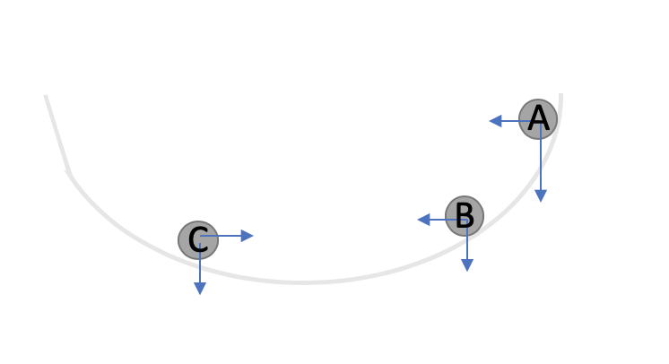
As compared to Batch Gradient Descent, Mini Batch is much faster. But it still leaves room for improvment. Think of a ball rolling down the hill. As long as the ball is rolling in one direction, it gains velocity but as soon as it changes direction, it’s velocity reduces. Another way to think about this is looking at component vectors of the gradient as shown in the image below. Let’s assume we computed the gradient at pt A and then pt B. If we look at the component vectors of the gradient at the two points, the two are in the same direction and thus it indicates that we are going in the right direction and ideally should move even more faster. But as we move from point B to C, the horizontal component vector are in the opposite direction and therefore indicates that we should now slow down.
Thus, one idea is to adjust the vector scomponents of the gradient based on the previously observed values of the gradient. In Momentum gradient descent, we use exponentially average. Essentially, the last observed gradient descent has the weight of \(\beta\). The one before that has the weight of \(\beta^2\) and so on. In other words, the effective gradient is computed in the following manner:
Below is the python implementation of the momentum gradient descent algorithm. Note that most of the logic is same except that we have an additional parameter, momentum, and an additional step to take exponential average of gradient.
from copy import copy
from random import random
from IPython.display import HTML
from tqdm import tqdm, trange


def momentum(X, y, learning_rate = 0.09, momentum = 0.9,
                        max_epoch = 1000, traceback = None, stopping_threshold = 1.0e-6
                        , starting_point = None
                        , num_batches = 10):
    """Minimizes
    momenutum -- how much weight historical gradient should carry. A good default value is 0.9
    """
    if 1 < momentum < 0:
        raise ValueError("Momentum should between 0 and 1")

    # number of samples
    m = X.shape[0]

    # number of parameters
    n = X.shape[1]

    # idx
    indexes = list(range(m))

    # starting point -- randomly select
    theta1 = np.array([random() for i in range(n)]) if starting_point is None else starting_point
    grad = np.zeros(n)

    for iter in trange(max_epoch):

        if traceback is not None:
            traceback.add(iter, theta1, mse(X, y, theta1))

        # create batches
        np.random.shuffle(indexes)
        for batchIdx in np.array_split(indexes, num_batches):

            bX = X[batchIdx]
            by = y[batchIdx]

            #========================================
            # Instead of taking the gradient, we compute
            # exponetial average gradient
            #========================================
            grad = (momentum * grad) + (1 - momentum) * gradient(bX, by, theta1)
            theta2  = theta1 - learning_rate * grad

            # check if we reached stopping criteria threshold

            if np.linalg.norm(grad) < stopping_threshold:
                print("Early Stopping at Iteration Number: ", iter)
                return theta2

            theta1 = theta2

    # if we reached max iterations then return current point
    return theta1


tracebacks['Momentum'] = Traceback('Momentum', 3)
theta = momentum(X, y, learning_rate=0.009,
                          momentum=0.9,  max_epoch=1000, traceback=tracebacks['Momentum'],
                          stopping_threshold=1e-6, starting_point=starting_point)

display(HTML("<strong>Optimized Parameters: {}</strong>".format(theta)))


plotCost(tracebacks.values(), min_iter=10, max_iter = 40, exclude=['BatchGradientDescent'])
0%| | 0/1000 [00:00<?, ?it/s]
23%|██▎ | 233/1000 [00:00<00:00, 2322.94it/s]
43%|████▎ | 427/1000 [00:00<00:00, 2191.43it/s]
64%|██████▎ | 636/1000 [00:00<00:00, 2158.39it/s]
87%|████████▋ | 873/1000 [00:00<00:00, 2216.68it/s]
100%|██████████| 1000/1000 [00:00<00:00, 2146.74it/s]
RMSPROP
RMSProp was one of the major development and fueled the growth of deep learning. While momentum leveraged historical gradients to speed up the gradient descent algorithm, one still has to provide right learning rate. RMSProp addresses this problem by automatically adjusting learning rate along each component of the gradient descent. You can find a good introduction of the methodology over here. The key equations are:
and
where \(\eta\) is the provided learning rate and \(\hat{\eta}\) is adjusted learning rate
from copy import copy
from random import random
from IPython.display import HTML
from tqdm import tqdm, trange


def rmsprop(X, y, learning_rate = 0.9, momentum = 0.9,
                        max_epoch = 1000, traceback = None, stopping_threshold = 1.0e-6
                        , starting_point = None
                        , num_batches = 10):
    """Minimizes
    X -- data frame containing X1 and X2
    y -- actual output values
    learning rate
    max_iterations
    traceback -- keep track of parameters
    stopping_threshold -- max distance between previous and new parameters at which it the algorithm should stop.
    """
    if 1 < momentum < 0:
        raise ValueError("Momentum should between 0 and 1")

    # number of samples
    m = X.shape[0]

    # number of parameters
    n = X.shape[1]

    # idx
    indexes = list(range(m))

    # starting point -- randomly select
    theta1 = np.array([random() for i in range(n)]) if starting_point is None else starting_point
    grad = np.zeros(n)
    grad2 = np.zeros(n)


    for iter in trange(max_epoch):

        if traceback is not None:
            traceback.add(iter, theta1, mse(X, y, theta1))

        # create batches
        np.random.shuffle(indexes)
        for batchIdx in np.array_split(indexes, num_batches):

            bX = X[batchIdx]
            by = y[batchIdx]


            # compute average gradient for all data points
            # and move in the opposite direction
            grad = gradient(bX, by, theta1)
            grad2 = (momentum * grad2) + (1 - momentum) * grad * grad
            weight = (learning_rate / (np.sqrt(grad2) + 1e-10)) * grad
            theta2  = theta1 - weight


            # check if we reached stopping criteria threshold

            if np.linalg.norm(grad) < stopping_threshold:
                print("Early Stopping at Iteration Number: ", iter)
                return theta2

            theta1 = theta2

    # if we reached max iterations then return current point
    return theta1


tracebacks['RMSProp'] = Traceback('RMSProp', 3)
theta = rmsprop(X, y, learning_rate=0.9, momentum=0.9,
                max_epoch=1000, traceback=tracebacks['RMSProp'],
                stopping_threshold=1e-6, starting_point=starting_point,
                num_batches=10)

display(HTML("<strong>Optimized Parameters: {}</strong>".format(theta)))

plotCost(tracebacks.values(), min_iter=0, max_iter = 50, exclude=['BatchGradientDescent'])
0%| | 0/1000 [00:00<?, ?it/s]
21%|██ | 212/1000 [00:00<00:00, 2113.51it/s]
42%|████▎ | 425/1000 [00:00<00:00, 2116.83it/s]
60%|██████ | 602/1000 [00:00<00:00, 1997.72it/s]
79%|███████▊ | 786/1000 [00:00<00:00, 1944.86it/s]
100%|█████████▉| 997/1000 [00:00<00:00, 1990.91it/s]
100%|██████████| 1000/1000 [00:00<00:00, 1983.14it/s]
Conclusion
In this chapter, I touched few of the variants of gradient descent algorithm. While RMSProp tends to often perform better, certain situations might require a different variants such as NAD, Adam, etc. A good summary of different variants of gradient descent is available over here. Below table summarizes key consideration points for different variants.
| Algorithm | Parameters | Advantages | Issues |
|---|---|---|---|
| Stochastic Gradient Descent (SGD) | learning rate, max epoch |
|
|
| Batch Gradient Descent | learning rate, max epoch |
|
|
| Min Batch Gradient Descent | learning rate, max epoch, either number of batches or batch size |
|
|
| Momenutm Gradient Descent | learning rate, max epoch, either number of batches or batch size, momentum (=0.9 by default) |
|
|
| RMSProp | learning rate, max epoch, either number of batches or batch size, momentum (=0.9 by default), \epsilon(=1.0e-6 by default) |
|
|
TODO
RMSProp shows significant improvement over all the previous versions of the gradient descent. But doesn’t converge as compared to other variants. Below plot shows MSE for the different algorithms.
plotCost(tracebacks.values(), min_iter=900, max_iter = 1000)